Methods for Measuring Resolution
and 50% MTF
Resolution
Resolution
tests were run at variable working distances from the target as calculated
from the Koren lens chart method. An
Edmund Scientific lens resolution chart with several overlain Koren 2003
lens test charts at different angles was illuminated with two
tungsten modeling bulbs from monolight flashes. The lenses were mounted on
a Bogen 3033/Arca Swiss B1 tripod/head combination with a large Kirk bean
bag weighing down the tripod/head to dampen vibration. Two to 5 exposures
using aperture priority exposure and +1.3 exposure compensation were taken
at each aperture with an EOS-1Ds Mark II via cable shutter release and in
mirror lockup mode at ISO 100 in RAW mode. The central autofocus point was
centered over the center pattern for each exposure. The lens was
defocused, and then refocused using autofocus for each exposure. RAW files
were converted to 300 dpi tifs with Phase One dslr software and images
were analyzed in Photoshop.
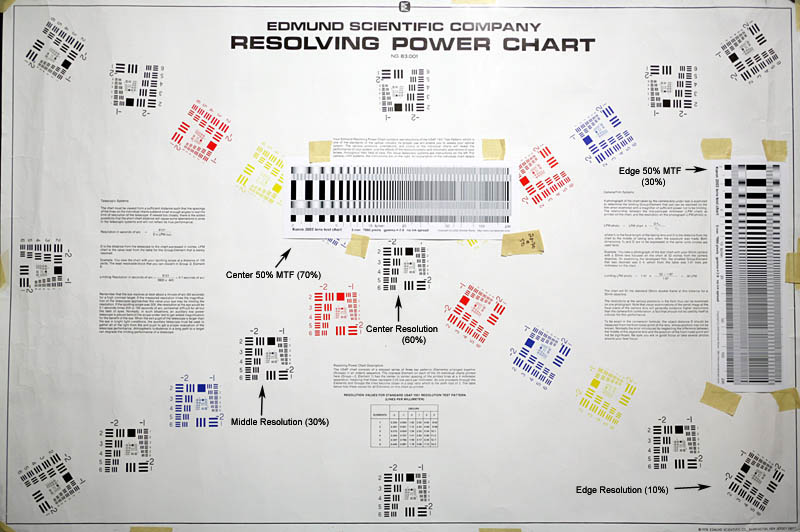
Measurement were made at the center pattern, a middle pattern, and the
edge pattern as shown here.
Both line patterns at 90° angles had to be clearly visible. The
highest resolution score for each aperture was recorded to minimize the
the effect of potential autofocus error. Center-weighted resolution was
calculated (60% center; 30% middle; 10% edge). Resolutions (lpm) at each
f/stop were calculated using the method on the chart as follows.
Image lines pairs per mm (image lpm or lp/mm) = lpm resolved on chart X
(D-fo) / fo) where fo = focal length of lens and D = Distance from the
chart to the middle of the lens.
50% MTF (modulation transfer
function):
There is general agreement that perceived image
sharpness is more closely related to the spatial frequency (lp/mm) where
MTF is 50% (i.e., where contrast has dropped by half) than to resolution
alone. I used the Koren 2003 lens test chart
developed
and explained by Norman Koren to calculate 50% MTF. Printed test
charts were placed on the Edmund Scientific Test Chart as in the middle
and edge of the chart as shown
here. The chart was photographed under tungsten bulb lighting from
two modeling lights. A Canon EOS-1Ds Mark II was set at ISO 100, tungsten
bulb white balance and shot with + 1.33 EV using evaluative metering with
the camera set for mirror lockup. Raw files were converted to 300 dpi tifs
with Capture One Pro v. 3.76. Measures of 50% MTF were calculated using a
centered weighted pattern (70% center, 30% edge).
The
imaged sine patterns were analyzed withand measurements were made on the
resulting Plot Profile to determine line pair per mm frequency of 50%
contrast as explained in detail on the Norman Koren website.
Details of calculating 50% MTF:
1. The 5mm Koren 2003 lens test chart designed to be printed at 25 cm
long (50X magnification) was downloaded from the Koren website and printed
on semi-gloss paper with a Epson 1270 printer at 1440 dpi. Charts are
trimmed and mounted on the Edmund Scientific Test Chart as shown:
2.
The chart is photographed at a working distance that is 1/2 the
recommended distance so that the entire Edmund Scientific chart can be
photographed for resolution and determination of 50% MTF. It is also
possible to detect lateral chromatic and other aberrations from the same
test images. The distance from the chart was calculated at d1=(M+1)f
where d1 = lens to target distance (mm) and f = lens
focal length (mm) and M=25. The reduction of distance by 1/2 requires that
lp/mm figures read off the chart be adjusted by 1/2.
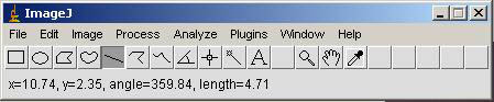
3.
Photographic RAW files are converted to tifs with Capture One Pro. The tif
files are opened in image analysis software to analyze the sine patterns
on the chart (top band). I used
ImageJ
software, public domain software off the NIH site.
Click on "File" and then "Open" to select and open the
tif of interest.
4. Click on the "magnifying cursor symbol"
to fill the window with the Koren chart image and click on the "hand"
icon to move the chart image into the middle of the window.
5.
Click on the line icon and draw a straight line through the upper sine
pattern bar on the Koren chart.

6.
Click on the "Analyze" menu and select "set scale" and
enter "known distance" as "25" and "units"
as "cm".
7. Click on "Analyze" again and
select "Plot Profile."
8. A sine wave pattern will be
generated and displayed.
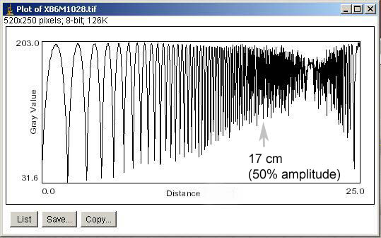
9.
The full amplitude of the sine wave on my computer screen has a 7 cm
sweep. I just take a rule and run it down the plot towards 25cm until the
amplitude is 50% (3.5 cm). In the example, 50% amplitude is at 17 cm on
the chart. This corresponds on a plot of cm of chart versus a log plot of
spatial frequency below to 47 lp/mm.
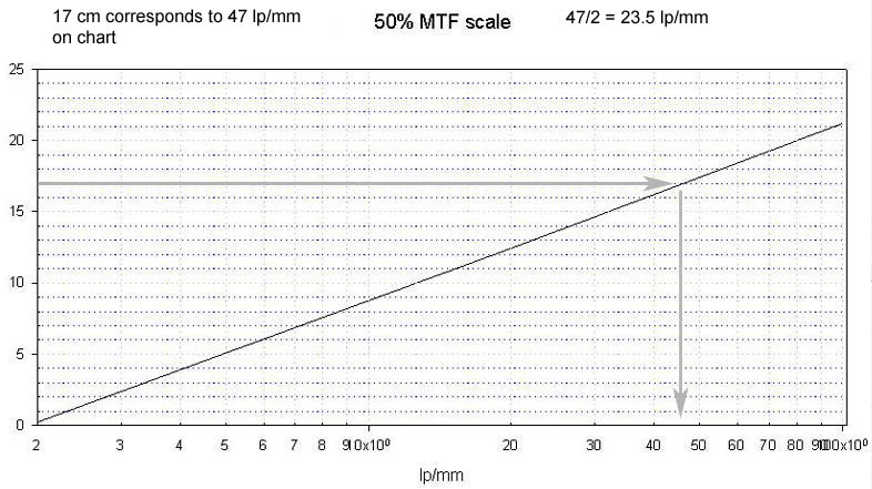
10.
Because the working distance was decreased by 1/2 when photographing the
chart, the lp/mm value is divided by 2 to generate the 50% MTF value.